What are the common statistical mistakes?
- Absence of an adequate control condition/group
- Interpreting comparisons between two effects without directly comparing them
- Spurious correlations
- Inflating the units of analysis
- Correlation and causation
- Use of small samples
- Circular analysis
- Flexibility of analysis
- Failing to correct for multiple comparisons
- Over-interpreting non-significant results
This is a visual summary of the 2019 eLife article “Ten common statistical mistakes to watch out for when writing or reviewing a manuscript” by Makin and Orban de Xivry.
If you’d prefer, you can watch the 5 minute video summary below:
This entire page is also available as a Twitter thread:
10 statistical mistakes in 5 min
— Stuart McErlain-Naylor (@biomechstu) April 6, 2021
"Ten common statistical mistakes to watch out for when writing or reviewing a manuscript"
5 min video summary: https://t.co/Vgi5h1oyYK
Thread below (1/16)
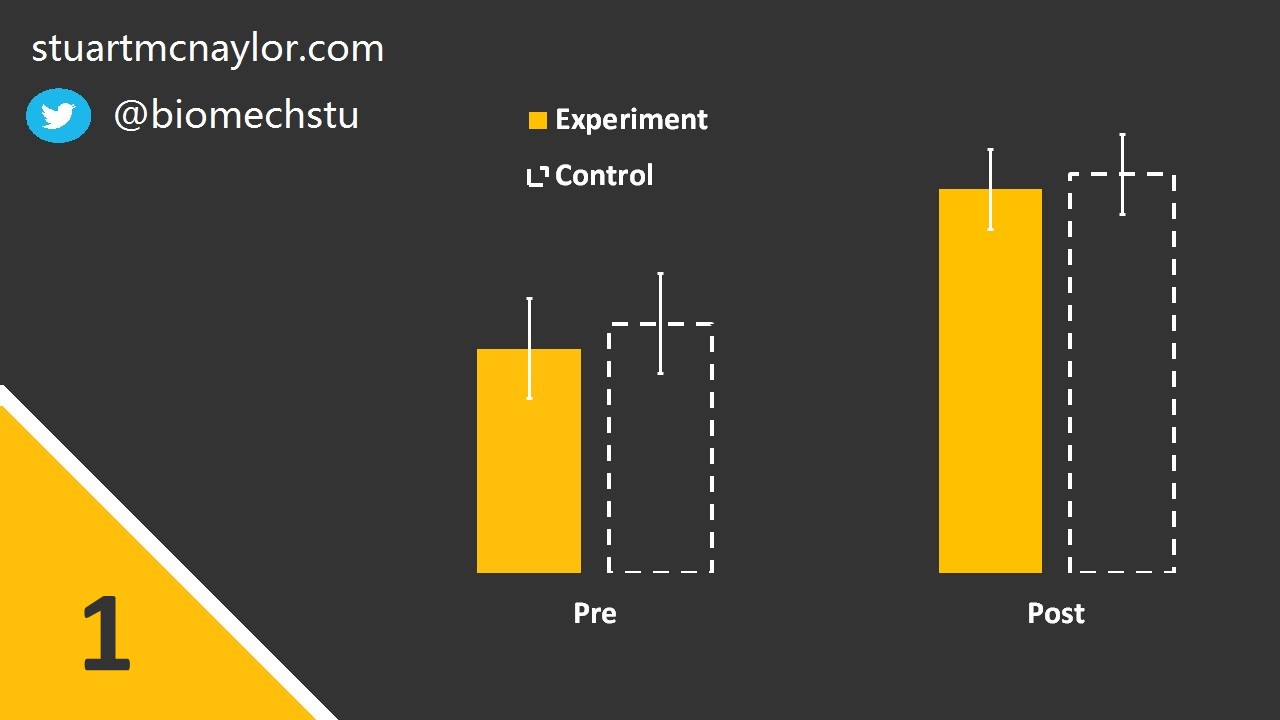
Mistake 1: Absence of an adequate control condition/group
The effectiveness of any intervention (or a change in any group) should not be judged in isolation.
The research should include an appropriate control condition/group against which the effect can be assessed.
Simple example: How do we know your intervention caused the athletes’ acute improvement in strength and that it wasn’t a result of other factors that would have happened even without the intervention?
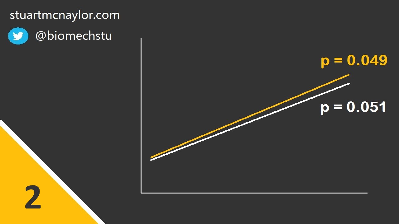
Mistake 2: Interpreting comparisons between two effects without directly comparing them
In our example above, we wanted to know if the intervention had a significantly greater effect on strength compared to a control condition.
To do this, we must directly compare the two effects. We cannot simply perform separate pre-post comparisons on each group and compare the p-values from the two statistical tests.
Simple example: Group 1 has a p-value (pre-post comparison) of 0.049 and Group 2 has a p-value of 0.051. You would therefore reject the null hypothesis of no change for Group 1 but not for Group 2. However, this doesn not mean that the effect for Group 1 is significantly greater than the effect for Group 2. In order to determine whether the two effect sizes were significantly different, you would need to directly compare them in a single test.
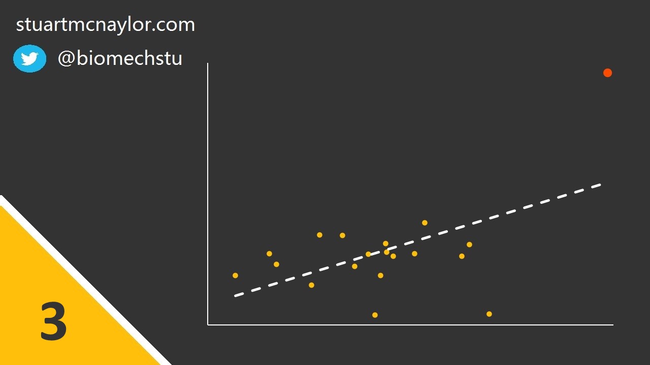
Mistake 3: Spurious correlations
Spurious correlations may occur in the presence of one or more outlier data points (see image below).
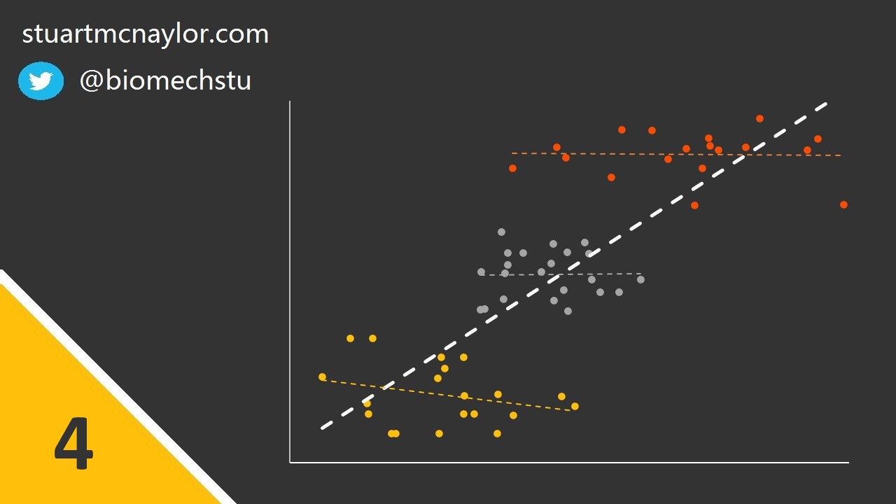
Additionally, this can occur when data from two or more sub-groups are combined - particularly when the observed correlation is not present within any of the sub-groups alone.
Simple example: Although there is no relationship between body mass and shooting accuracy, one player is much heavier than the rest of the squad and is also the best shooter. This player skews the overall relationship, resulting in a spurious correlation between the two variables.
Mistake 4: Inflating the units of analysis
The greater the degrees of freedom in a test, the lower the critical size of effect that would be considered significant. Anything that falsely inflates the degrees of freedom can therefore increase the likelihood of false positive results.
This can often occur when multiple trials by multiple participants are all compared within a single comparison (i.e. merging within-participant variation and between-participant variation). The within- and between-participant effects should be assessed as separate effects.
Simple example: You have 20 participants, each performing 3 countermovement jumps. In your correlation analysis, you include all 60 data points as if they are all independent from each other (they are not).
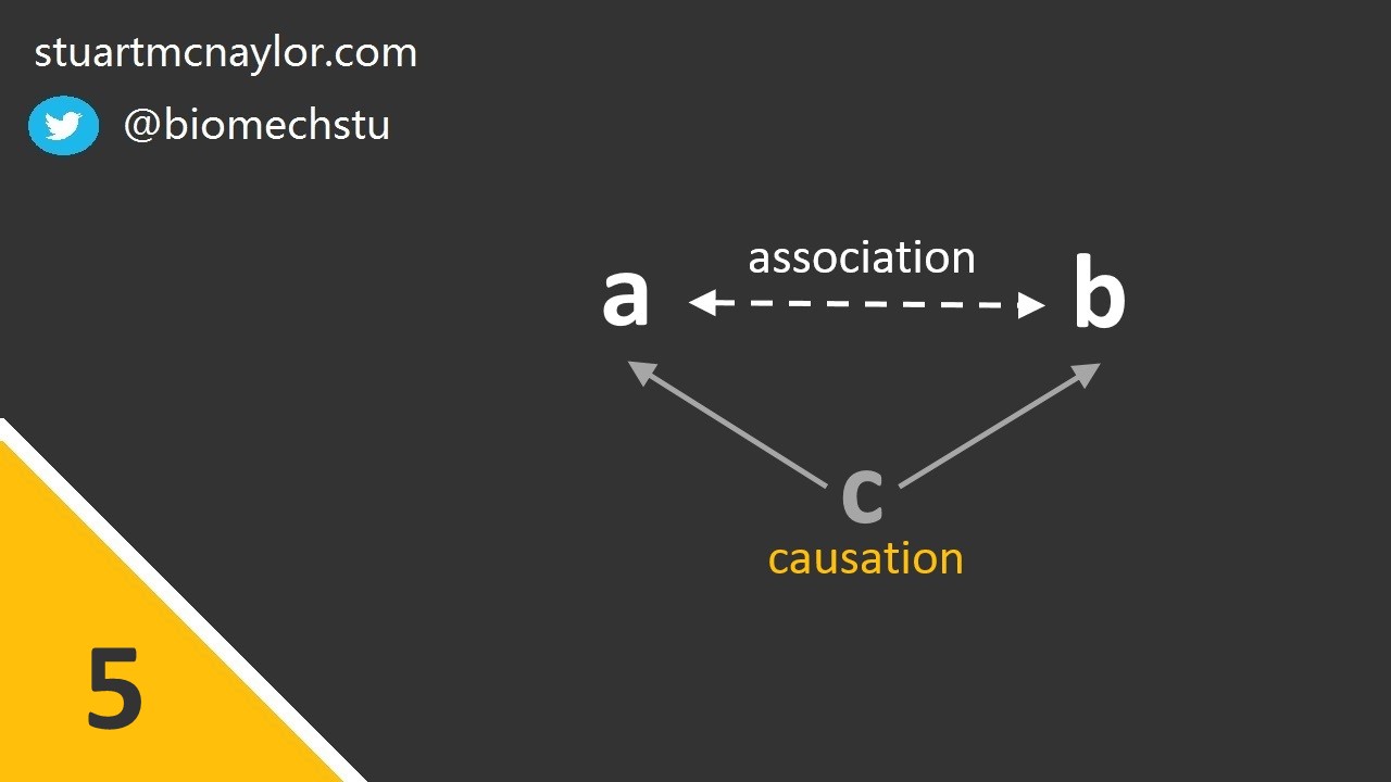
Mistake 5: Correlation and causation
We should not assume that all correlations are cause and effect relationships.
In reality, we can only make this assumption when the correlation is the direct result of an intervention. Even then, we should be cautious about the presence of confounding variables. It may be preferable to use the term ‘is associated with’ rather than ‘causes’ or ‘results in’.
Simple example: You report a significant correlation between sprint speed and passing accuracy in a team sport. You can correctly state that there is an association between the two variables. However, you should not claim that greater sprint speeds cause greater passing accuracy. Instead, it may be that both factors are related to a third variables such as training experience.
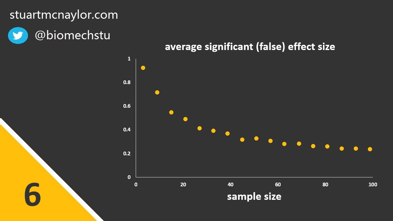
Mistake 6: Use of small samples
The greater the sample size, the lower the critical size of effect that would be considered significant. The smaller the size of effect you wish to observe (assuming the effect exists; for example, the smallest effect that would be considered practically or clinically significant), the more participants you will need to reliably observe that effect. For more on sample size calculations, see my 5 minute demonstration of G*Power power analysis (no prior experience required):
The smaller the sample size, the greater the average effect size of false positive results (i.e. those that result in significant results due to chance, despite the null hypothesis actually being true in the population). We should therefore avoid the trap of thinking that despite our small sample size, our results must be true due to their large effect size.
Simple example: Despite your sample size of only 10 participants, you observe a ‘large’ effect size and so you falsely conclude that your small sample wasn’t an issue.
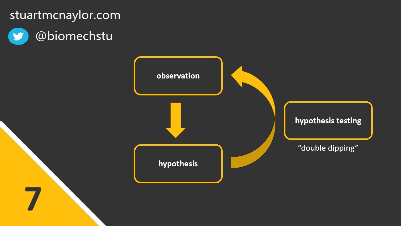
Mistake 7: Circular analysis
This is sometimes called “double dipping”.
We should always test our hypotheses on a separate sample to the one that led to the generation of the hypotheses in the first place. Otherwise, any hypotheses formed due to chance patterns in the data are likely to be confirmed when the same data is used to assess those hypotheses.
Likewise, simulation models should be evaluated against different trials to the ones used to determine model parameters.
Simple example: You fail to reject your original null hypothesis but you spot something in your data that leads you to form a second possible explanation. You test this new hypothesis statistically on the same data and confirm your suspicion.
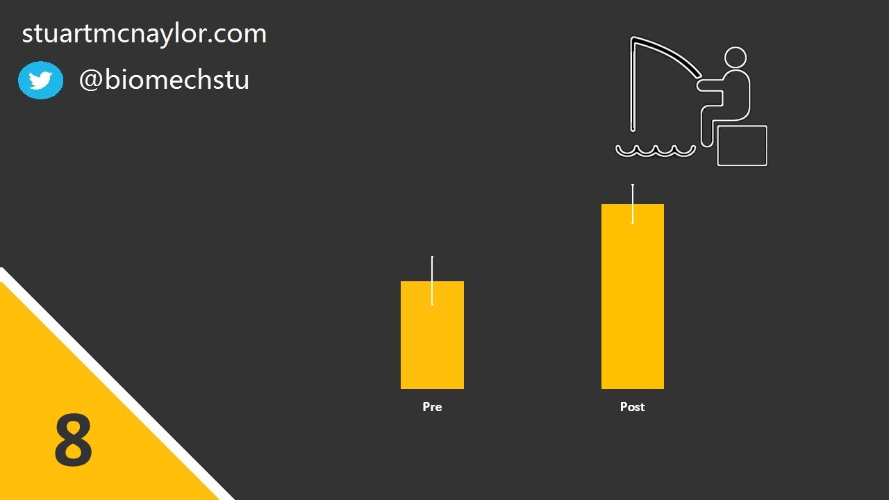
Mistake 8: Flexibility of analysis
You may have heard the term ‘p-hacking’. This is where researchers utilise flexibility in their analysis plans to search for possible significant effects or lower the p-value of observed effects.
Some examples include the removal of individual data points, testing of alternative hypotheses and dependent variables, or the unjustified use of a one-tailed hypothesis test. Similarly, researchers may change the criteria against which a simulation model is evaluated.
Many open science practices are aimed at preventing p-hacking, among other issues affecting replicability of research findings. This includes pre-registration and registered reports, both of which involve registering the analysis plan prior to the collection of data.
Simple example: You calculate a p-value of 0.06, but realise that it would be significant if the oldest participant was removed. Surely that was an error in your exclusion criteria, right? Or maybe you’ve just decided a one-sided test would have been fine after all? Or maybe that wasn’t actually the hypothesis you wanted?
Mistake 9: Failing to correct for multiple comparisons
The more variables you test, the more likely it is that one of them will correlate significantly with your dependent variable by chance, even if the null hypotheses are all true in the population.
It is therefore necessary to correct for multiple comparisons. Possible approaches include the Bonferroni, Benjamini and Hochberg, or Holm’s step-down adjustment methods.
Simple example: You measure 40 different parameters during a jump and assess the correlation of each variable against jump height. A small number of variables correlate significantly but no correction has been performed for the multiple tests.
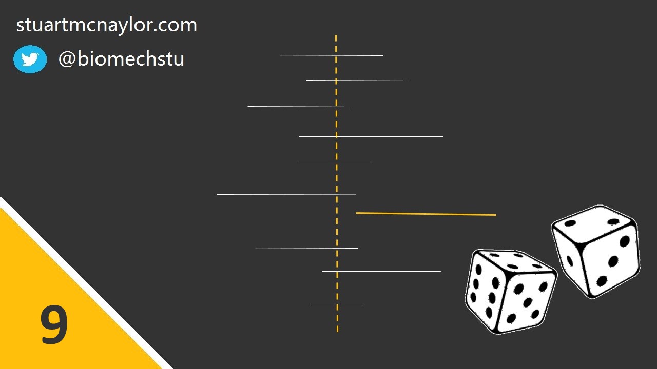
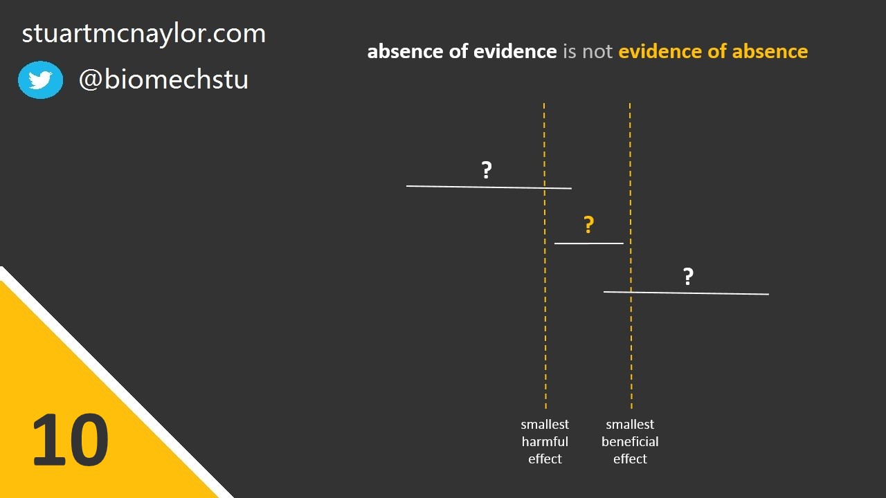
Mistake 10: Over-interpreting non-significant results
Absence of evidence is not evidence of absence.
So you failed to reject the null hypothesis. This does not mean that you are accepting the null hypothesis as correct, just that you didn’t reject it.
A 95% frequentist confidence interval represents the range of effect sizes that would not be rejected at p < 0.05. You should therefore not reject any of the effect sizes within that range (including the null but also possibly including some meaningful effect sizes).
Simple example: You calculate a p-value of 0.06, with the confidence interval including large positive effects but also some very small negative effects. You cannot reject the null hypothesis but you should also not reject the possibility of a meaningful positive effect.
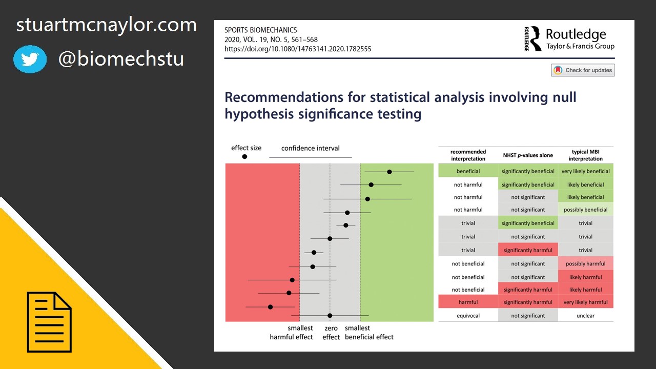
More information
For more on the use of effect sizes and confidence intervals to make inferences, see our editorial in Sports Biomechanics on ‘Recommendations for statistical analysis involving null hypothesis significance testing’:
For a full lecture on fundamental statistical concepts, taught using visualisations and simulations, check out Kristin Sainani’s lecture as part of the Sports Biomechanics Lecture Series:
For more free online resources on statistics and other aspects of academia, please take a look at the resources section of my website.
With new PhD students starting today, I compiled a list of 𝗳𝗿𝗲𝗲 𝗼𝗻𝗹𝗶𝗻𝗲 𝗿𝗲𝘀𝗼𝘂𝗿𝗰𝗲𝘀 that I've found particularly useful.
— Stuart McErlain-Naylor (@biomechstu) October 1, 2020
🔗 https://t.co/y9fbbfHsbv
I'll keep adding to this, so let me know if you have any favourites!#AcademicChatter #AcademicTwitter #phdchat pic.twitter.com/rr86ctJYTd
Finally, for monthly updates on any new resources, content, or research articles, please sign up to my newsletter: